Set Continuous Data Axis Google Sheets

Learning how to create dot plots in Google Sheets is useful for creating a simple and easy-to-understand representation of data.

Dot plots are graphical displays that use dots to represent data.

When working with data, there may be instances where you will need to present your findings to an audience. Common ways of summarizing data are through the use of tables or graphs. While tables provide a more detailed summary of data, graphs are more readily understood as they give numbers shape and form.

Of all the available graph/chart types, a dot plot (or dot chart) is one of the simplest and easiest to understand. From its name, dot plots use dots to represent data.

You may be wondering how dot plots differ from scatter plots or bubble charts. Are they even different or are they just the same? Dot plots are used for representing univariate data: data with only one variable being considered. Scatter plots consider two variables, where the position of each dot on the x and y-axis indicates the value of that data point. Bubble charts expand on the scatter plot by adding another variable to consider. The value of this additional variable is presented by varying the size of each dot.

What instances are dot plots the best option for presenting data? Dot plots are especially useful when the variable is categorical or quantitative. Categorical variables are those that can be organized into categories: music genres, brands, types of materials, etc. On the other hand, quantitative variables are variables that can be measured and have numerical values.

In this article, we shall be discussing different types of examples and the different ways of creating dot plots based on the type of the variable used. Each has its specific uses and advantages on the way data is presented.

Consider this first example.

A Real Example of Frequency Type Dot Plots

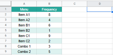
Suppose you are given the task of conducting a survey to see which menu item is the tastiest in a certain restaurant. Afterward, you are to present your findings in the form of a dot plot. The results of the survey are as follows:

The situation above is an example of data whose variable considers the frequency of a given categorical item. Survey data is one of the most common frequency types of data used in making dot plots. Other data whose variables represent a count of each item may also be considered under this type.

Now, let's learn how to create a dot plot for this type of data!

How to Create Frequency Type Dot Plots

Google Sheets have various chart types that you can use to quickly insert graphs. However, dot plots are not one of the chart types available. The closest similar types are the scatter chart and bubble chart. For this tutorial, we shall be learning how to use the scatter chart to create dot plots.

Visit our tutorial on How to Add a Chart and Edit the Chart Legend in Google Sheets if you are still not familiar with how to insert charts in Google Sheets.

For frequency type dot plots, each dot in the graph represents the count for each item. This tutorial will be making use of two functions, namely, ARRAYFORMULA and SEQUENCE functions. Follow the links to each function for more detailed discussions.

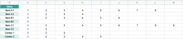
1. Since each dot will represent a data point, we need to create a new table for the chart to extract data from. Simply click on any cell to make it the active cell. For this guide, I will be selecting D1, where I want to show my result.

2. Next, simply type the equal sign '=' to begin the function. To copy the contents of column A, select cell A1, press and hold the Shift key, then select A9. Notice that all the cells from A1 to A9 are selected and the text in the formula shows "A1:A9". This range should cover all of the categories you have.

3. To change this formula into an ARRAYFORMULA, press the Ctrl+Shift+Enter keys. This will add the ARRAYFORMULA function to the formula. You can also manually type this function into the formula.

4. Press Enter to finish the formula. Notice that cells below D1 are filled with the values from column A even though we only put a formula to cell D1. Next, select cell E2. We will now insert the sequence formula "=SEQUENCE(1,B2)". Copy this formula to all the items considered. Notice that for each column, the number increases by 1 until the value of the frequency is reached.

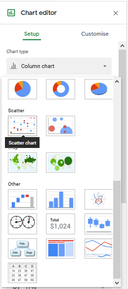
5. To insert a chart, first, specify the data on which our chart will be based on. Select the range D1:M9. Go to the upper menu and select Insert > Chart. From the Chart editor toolbar at the right, change the chart type to a scatter chart.

6. You should end up with the following graph. To make sure that the graph created is correct, the range in the X-axis should be the items in column D. The values in the series portion should be multiple ranges. Each range should correspond to each column from E to M. The 'Use column D as labels' option should also be ticked. If you choose to have headers put in cells E1:M1, also make sure that the 'Use row 1 as headers' option is checked. Notice how for each value in the vertical axis, the same color is used in all of the categories (a count of 1 is blue, 2 is red, and so on).

7. You may remove the legend if you wish, just select the colored dots at the side and press the Delete key. To end up with a traditional looking dot plot, labels for the y-axis (frequency) should not be present. Unlike the legend, this cannot be deleted. Just mask it by changing the text color to white. Select the labels of the vertical axis. This will take you to the Customise tab of the Chart editor toolbar. Under 'vertical axis', set the text color to white.

8. Following the steps above should lead you to the following dot plot. Further customization can be made in the Customise tab.

This type of dot plot is similar to a histogram where it displays the number of data points that fall into each category/value on the vertical axis. Since the only labels present in this type of dot plot are the categories, viewers need to manually count each dot to know the exact frequency of each item. Therefore, this type of dot plot is most suited for data with a small number of values. For larger data sets, other types of charts like histograms or box plots are more useful.

That's pretty much all you need to know to create frequency type dot plots! Now, let's consider another example with a different type of data.

A Real Example of Comparative Type Dot Plots: Discrete

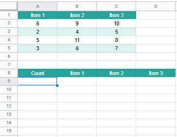
You are to determine which among 3 items is the best selling product of a given store. Basing off of a single day's sales would not give an accurate conclusion as sales for each product fluctuates. You decided to take the number of sales of each product for 4 days and visualize this data through a dot plot. The data is presented below:

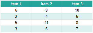
The situation above is an example of data that changes over time. For this segment, we shall focus first on discrete types of data, specifically, values that are integers. Other data whose variables change and need to be compared may also be considered under this type.

We shall call a dot plot that has this kind of data as comparative type dot plots. Now, let's learn how to create a dot plot for this type of data!

How to Create Comparative Type Dot Plots: Discrete

This tutorial will be making use of multiple functions which include the two functions included before (ARRAYFORMULA and SEQUENCE), along with additional functions such as MAX, MIN, IFNA, and VLOOKUP. MAX and MIN function returns the maximum and minimum value in a given range, respectively. IFNA is a more specific version of the IFERROR function, where the type of error considered is the #N/A error.

Follow the links to each function for more detailed discussions.

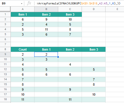
1. First, we need to create a new table for the chart to extract data from. This table shall contain columns pertaining to the count and each category being considered. Simply click on any cell to make it the active cell. For this guide, I will be selecting A9 where I want to show my result.

2. Next, type "=SEQUENCE(MAX(A2:C5)-MIN(A2:C5)+1,1,MIN(A2:C5))", then press the Enter key. For different sized data sets, replace A2:C5 in the formula with the range corresponding to the numerical values in the data set. Notice that for each row, the number starts from the minimum value, then increases by 1 until the maximum value is reached.

3. Next, type "=ArrayFormula(IFNA(VLOOKUP($A$9:$A$18,A2:A5,1,0),))" in cell B9. Copy this formula to all the items considered (C9:D9).

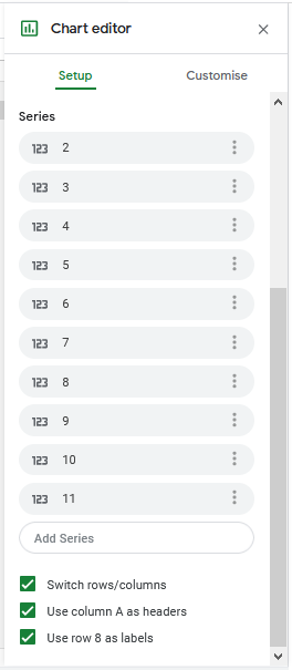
4. To insert a chart, first, specify the data on which our chart will be based on. Select the range A8:D18. Go to the upper menu and select Insert > Chart. From the Chart editor toolbar at the right, change the chart type to a scatter chart. Check the boxes for 'Switch rows/columns', 'Use row 8 as headers', and 'Use column A as labels'.

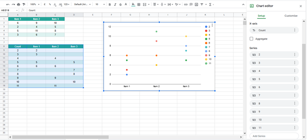
5. You should end up with the following graph.

6. To make sure that the graph created is correct, the range in the X-axis should be the items in row 8. The values in the series portion should be multiple ranges. Each range should correspond to each row from 9 to 18. Similar to the earlier example, for each value in the vertical axis, the same color is used in all of the categories (a count of 2 is blue, 3 is red, and so on).

7. Further customization can be made in the Customise tab. Feel free to change whatever you like from the color of the data series, size, and shape of the dots, text fonts, etc. Since we already have labels on the vertical axis, let's remove the legend. Following the steps above should lead you to the following dot plot.

The comparative type dot plot is most useful when trying to visualize relative values of one category to another. Looking at the example, we can see that Item 1 has generally the lowest sales, while Item 3 has generally the highest. Although there are days where Item 2 sells out more than Item 3, its general sales tend to fluctuate by a large margin.

The process described for creating this type of dot plot will only work if the data set is made up of discrete values with a common difference. This is due to the use of the SEQUENCE function. What if our data set is made up of continuous values? Decimals and fractions are still quantitative variables, and thus, could still be presented in a dot plot. So how exactly can we do that?

Let's look at the last example.

A Real Example of Comparative Type Dot Plots: Continuous

Suppose you are to determine and compare the sales generated by three of your employees over the past 4 years. You are to present your findings and have decided to use a graph so that your audience can better interpret the data you have collected. The data is presented below:

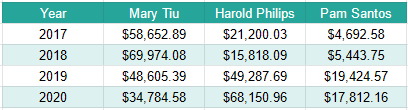
Similar to the second example, variables concerning items grouped into categories change over time. This time, however, the data set are decimal values, not integers. They have no common difference and vary widely. Using the approach of the second example will not be practical as the sequence function cannot be used. How should we tackle this problem? Let's find out below!

How to Create Comparative Type Dot Plots: Continuous

Unlike the previous examples, this method of creating a dot plot will not make use of additional functions. An additional table where the dot plot will extract data will also not be necessary.

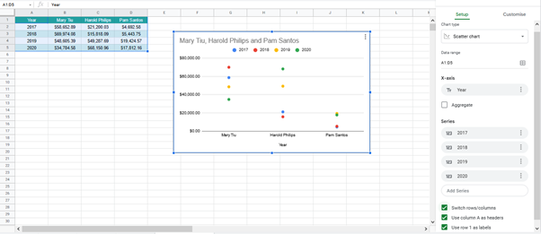
1. First, specify the data where our chart will be based on. Select the range A1:D5. Go to the upper menu and select Insert > Chart.

2. From the Chart editor toolbar at the right, change the chart type to a scatter chart. Check the boxes for 'Switch rows/columns', 'Use row 1 as headers', and 'Use column A as labels'. You should end up with the following graph.

3. To make sure that the graph created is correct, the range in the X-axis should be the items in row 1. The values in the series portion should be multiple ranges. Each range should correspond to each row from 2 to 5. They should also be labeled with the values in column A. Contrary to earlier examples, values placed in the same row of the table use the same color, not those of equal values.

4. Further customization can be made in the Customise tab. Feel free to change whatever you like from the color of the data series, size, and shape of the dots, text fonts, etc. For this graph, I'll remove the chart and x-axis titles, and move the legend to the right of the graph. Following the steps above should lead you to the following dot plot.

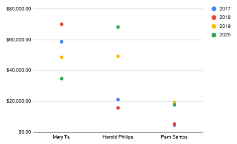
From the dot plot, we can see that Pam Santos generally has the lowest sales of the three and Mary Tiu has the highest, while Harold Philips's sales vary by a large margin.

Looking at how these dots are colored, we can also derive further conclusions. Blue and red dots represent the years 2017 and 2018, while yellow and green dots are for sales during 2019 and 2020. Despite Mary having the highest average sales, her yearly sales are generally declining. Meanwhile, Pam and Harold have improved since their early years, with Harold having a big boost in sales for the past years.

Now you may be wondering, why go through the process explained in the second example if this process is much simpler? Each process differs in how data is grouped. For the process with discrete values, those with equal values are grouped together. On the other hand, the process for continuous values group data based on how they are placed in the table. Depending on what you want to emphasize, one process may be better to use.

Of course, the process for continuous data may be used for discrete values. However, some tweaks should be applied to the process for discrete data for it to be applied to continuous data. These will not be further discussed but are presented in the spreadsheet that we will provide at the end of the article.

To ensure ease of creating dot plots in Google Sheets, take note of the following information for creating scatter charts:

• Only one range may be used in the x-axis. Multiple ranges may be considered for inputting the values in the y-axis. These ranges are called "Series" and each series is assigned a different color.
• By default, ranges considered are grouped by columns and the 'Use column X as labels' checkbox is ticked. This column is the first column in the data range specified and is automatically used as the values for the x-axis.
• The 'Use row 0 as headers' checkbox always considers the first row in the data set if headers are to be specified.
• Selecting the 'Switch rows/columns' checkbox shall reverse the way values are inputted into the chart. Ranges are now grouped by rows. Values considered as labels are now the first row in the data range. The checkbox for this also changes to 'Use row 0 as labels'. Similarly, headers considered are the first column in the data range when the 'Use column X as headers' checkbox is ticked.

We're finally done! This tutorial presented three ways of creating dot plots and discussed the uses of each one. If you want to practice some more, make a copy of our spreadsheet and give it a try:

Or browse our other numerous Google Sheets formulas to create even more powerful formulas that can make your life much easier.

Get emails from us about Google Sheets.

Our goal this year is to create lots of rich, bite-sized tutorials for Google Sheets users like you. If you liked this one, you'll love what we are working on! Readers receive ✨ early access ✨ to new content.

foxsheroattept.blogspot.com

Source: https://sheetaki.com/how-to-create-dot-plots-in-google-sheets/

Share this post